Workshops
The idea of the weekly workshop sessions is to go through some technical analytical exercises together. A pre-condition for a successful learning experience is that you stay on top of the weekly lecture material, otherwise the workshop exercises won’t make much sense to you.
Our weekly meetings are also an excellent opportunity for you to provide feedback and help me understand your priorities. Feel free to suggest topics that you would like me to cover. I’m more than happy to adapt the workshop to reflect your needs and preferences.
Please let me know if you have any other great ideas to turn the weekly workshops into a rewarding learning experience for you. Let’s be open minded throughout and have a continuous conversation on how to make the workshop suit your needs.
Week 1
No exercises in first week. Phew!
Week 2
Exercise 1
You have available a sample of \(n\) independently and identically distributed observations \(Y_1, Y_2, \ldots, Y_n\) (this is called a random sample). Let \(E(Y_1) = \mu\) and \(Var(Y_1) = \sigma^2\) where \(\mu\) and \(\sigma\) are placeholders for real numbers.
Now consider the following weighted average:
where \(n\) is an even number.
Derive the mean and variance of \(\widetilde{Y}\). Compare them to the mean and variance of \(\bar{Y}\).
Exercise 2
Assume that grades on a standardized test are known to have a mean of 500 for students in Europe. The test is administered to 600 randomly selected students in Ukraine; in this sample, the mean is 508, and the standard deviation is 75.
Construct a 95% confidence interval for the average test score for Ukrainian students.
Is there statistically significant evidence that Ukrainian students perform differently than other students in Europe?
Another 500 students are selected at random from Ukraine. They are given a 3-hour preparation course before the test is administered. Their average test score is 514, with a standard deviation of 65.
Construct a 95% confidence interval for the change in mean test score associated with the prep course.
Is there statistically significant evidence that the prep course helped?
Week 3
Exercise 1
This exercise provides an example of a pair of random variables, X and Y, for which the conditional mean of Y given X depends on X yet \(\rho_{XY} = 0\).
Let X and Z be two independently distributed standard normal random variables, and let \(Y=X^2+Z\).
What are \(E(X)\), \(E(X^2)\), and \(E(X^3)\) equal to?
Show that \(E(Y|X) = X^2\).
Show that \(E(Y) = 1\).
Parts 2 and 3 show: \(E(Y|X) \neq E(Y)\), that is, Y and X are not CMI.
Show that \(E(XY)=0\).
Show that \(Cov(X,Y)=0\) and therefore \(\rho_{XY}=0\).
In the lecture you learned that CMI of two random variables \(X\) and \(Y\) implies that their covariance and correlation are zero. It is important to understand that the converse of that statement is not true: zero covariance/correlation do not imply CMI.
Panel (d) of Figure 3.3 on page 130 of the textbook illustrates this point (page 140 if you are using the updated 3rd edition).
Exercise 2
Let’s do some least squares estimation.
You have i.i.d. observations \(Y_i\) for \(i=1,\ldots,n\). Your goal is to estimate the unknown population mean \(\mu_Y\). You have learned in the lecture that the best thing you can do is use the sample average (because it is BLUE). Nevertheless you ignore my advice from the lecture and you choose a different estimator instead.
You decide to use the least squares estimator
Arguing intuitively, what is this estimator doing? Does it seem sensible?
Mathematically derive the estimator. Is it unbiased? Is it efficient?
You can look in the textbook on pages 107-108 for clues (pages 115-116 if you are using the updated 3rd edition).
Week 4
Exercise 1
Prove the following two facts involving the sum operator. These two facts come in handy when deriving the OLS estimators from the first order conditions that result from the least squares objective function (see lecture notes 4).
\(\sum_{i=1}^n X_i = n \bar{X}\)
In words: the sum of the \(n\) values is equal to \(n\) times the average value.
\(\sum_{i=1}^n (X_i - \bar{X}) (Y_i - \bar{Y}) = \left( \sum_{i=1}^n X_i Y_i \right) - n \bar{X} \bar{Y}\)
Exercise 2
Establish the following algebraic facts about OLS:
The sum of all residuals is zero: \(\frac{1}{n} \sum_{i=1}^n \widehat{u}_i = 0\)
The average prediction is equal to the sample average: \(\frac{1}{n} \sum_{i=1}^n \widehat{Y}_i = \bar{Y}\)
Residuals and regressors are orthogonal: \(\sum_{i=1}^n \widehat{u}_i X_i = 0\)
You can look in the textbook on pages 175-176 for clues (pages 190-191 if you are using the updated 3rd edition).
Week 5
Show that \(\widehat{\beta}_0\) is an unbiased estimator of \(\beta_0\). (Hint: Use the fact \(\widehat{\beta}_1\) is unbiased.)
Week 6
Exercise 1
We are taking a closer look at the regression \(R^2\).
Show that TSS = ESS + RSS.
A simple linear regression yields \(\widehat{\beta}_1 = 0\). Show that \(R^2=0\).
Exercise 2
Consider the following alternative regression models:
where \(a\) and \(b\) denote nonzero constants.
Show that \(\widehat{\gamma}_1 = (a/b) \widehat{\beta}_1\) and that \(\widehat{\gamma}_0 = a \widehat{\beta}_0\).
Show that \(\widehat{\delta}_1 = \widehat{\beta}_1\) and that \(\widehat{\delta_0} = \widehat{\beta}_0 + ( a - b \widehat{\beta}_1)\).
(Note: in parts a) and b), Greek letters with hats denote OLS estimators.)
What are you learning here? Part a) shows that multiplying the data by constants does change both the OLS estimates of the slope \(\widehat{\gamma}_1\) and the intercept \(\widehat{\gamma}_0\). But this change is easy: just multiply the original OLS estimator by \(a/b\) (slope) or \(a\) (constant).
Part b) shows that when adding constants to the data, the slope estimate does not actually change at all, while the intercept shifts by \(a - b \widehat{\beta}_1\).
Week 7
Exercise
Consider the regression model
for \(i=1,\ldots,n\). Notice that there is no constant term here.
Write down the least squares objective function.
Obtain all partial derivatives.
Write down all first order conditions.
Derive an expression for \(\widehat{\beta}_1\) as a function of \(\widehat{\beta}_2\). Similarly for \(\widehat{\beta}_2\).
Suppose (only here) that \(\sum_{i=1}^n X_{1i} X_{2i} = 0\). Show that \(\widehat{\beta}_1 = \sum_{i=1}^n X_{1i} Y_i / \sum_{i=1}^n X_{1i}^2\).
Suppose that the model does include an intercept: \(Y_i = \beta_0 + \beta_1 X_{1i} + \beta_2 X_{2i} + u_i\). Show that \(\widehat{\beta}_0 = \bar{Y} - \widehat{\beta}_1 \bar{X}_1 - \widehat{\beta}_2 \bar{X}_2\).
Still suppose that the model does include an intercept. Also suppose that \(\sum_{i=1}^n (X_{1i} - \bar{X}_1) (X_{2i} - \bar{X}_2) = 0\). Show that \(\widehat{\beta}_1 = \sum_{i=1}^n (X_{1i} - \bar{X}_1) (Y_i - \bar{Y}) / \sum_{i=1}^n (X_{1i} - \bar{X}_1)^2\).
Week 8
We’ll first do a very quick run-through Assignment 1.
If you want more specific feedback, please talk to your tutor after the computer labs, or visit them during their regular consultation hours.
Exercise
A recent study found that the mortality rate for people who typically sleep fewer than 7 hours per night is 5 percentage points higher than for people who typically sleep more than 7 hours a night. The 1.1 million observations used for this study came from a random survey of Australians aged 30 to 102. Each survey respondent was tracked for 4 years, sleeping patterns and mortality outcomes were
observed over that 4 year period.
Based on this brief summary of the survey, would you recommend that Australians who sleep fewer than 7 hours per night should try to sleep longer as a way to prolonging their lives? Explain.
Week 9
The following exercise deepens your understanding of how functional form specifications (such as logarithms and interaction terms) affect the interpretation of the population regression function.
Suppose a researcher collects data on houses that have sold in a particular neighborhood over the past year and obtains the regression results in the following table.
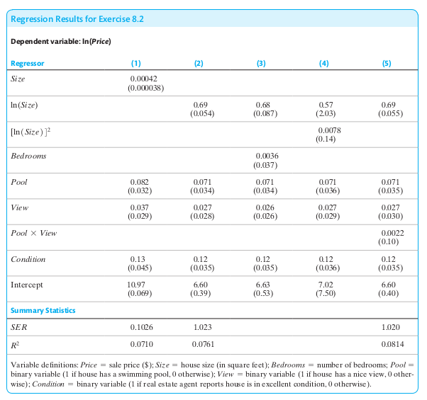
Using the results in column (1), what is the expected change in price of building a 1500-square-foot addition to a house?
How is the coefficient on ln(Size) interpreted in column (2)?
Is the interaction term between Pool and View statistically significant in column (5)? Find the effect of adding a view on the price of a house with a pool, as well as a house without a pool.
Week 10
The following two exercises provide a gentle introduction to the AR(p) model. The material to solve these two exercises should come straight out of this week’s lecture.
Exercise 1
Consider the AR(1) model \(Y_t = \beta_0 + \beta_1 Y_{t-1} + u_t\). Suppose the process is stationary. (Hint: A time series is stationary if its probability distribution does not change over time.)
Show that \(E(Y_t) = E(Y_{t-1})\).
Show that \(E(Y_t) = \beta_0/(1-\beta_1)\).
Exercise 2
The Index of Industrial Production \(IP_t\) is a monthly time series that measures the quantity of industrial commodities produced in a given month. This problem uses data on this index for the United States. All regressions are estimated over the sample period 1986:M1–2017:M12 (that is, January 1986 through December 2017). Let \(Y_t = 1200 \cdot ln (IP_t / IP_{t-1})\).
A forecaster states that \(Y_t\) shows the monthly percentage change in IP, measured in percentage points per annum. Is this correct? Why?
Suppose she estimates the following AR(4) model:
\[\widehat{Y}_t = \underset{(0.488)}{0.749} - \underset{(0.0088)}{0.071} Y_{t-1} + \underset{(0.053)}{0.170} Y_{t-2} + \underset{(0.078)}{0.216} Y_{t-3} + \underset{(0.064)}{0.167} Y_{t-4}\]Forecast the value of \(Y_t\) in January 2018, using the following observations:
Date
IP
Y
2017:M7
105.01
2017:M8
104.56
2017:M9
104.82
2017:M10
106.58
2017:M11
106.86
2017:M12
107.30
Week 11
Exercise 1
Suppose \(Y_t\) follows the stationary AR(1) model \(Y_t = 2.5 + 0.7 Y_{t-1} + u_t\) where \(u_t\) is i.i.d. with \(E(u_t) = 0\) and \(Var (u_t) = 9\).
Compute mean and variance of \(Y_t\).
Compute the first two autocovariances of \(Y_t\).
Compute the first two autocorrelations of \(Y_t\).
Suppose \(Y_T = 102.3\). Compute \(Y_{T+1|T} = E(Y_{T+1| Y_T, Y_{T-1}, \ldots})\).
Exercise 2
Suppose \(\Delta Y_t\) follows the AR(1) model \(\Delta Y_t = \beta_0 + \beta_1 \Delta Y_{t-1} + u_t\).
Show that \(Y_t\) follows an AR(2) model.
Derive the AR(2) coefficients for \(Y_t\) as function of \(\beta_0\) and \(\beta_1\).
Week 12
We’ll first do a very quick run-through Assignment 2.
After that, I will work through the practice exam.
This demonstration should address any concerns and questions that you have with regard to the level of detail required in answering questions and the possible degree of brevity you can use in formulating your answers.